RAG Pipeline Setup: Vector Database + LLM Integration Guide
Complete RAG pipeline tutorial with vector database setup, embedding strategies, chunking methods, and Python code examples using OpenAI, Chroma, and Qdrant.
RAGVector DatabasePythonLLMEmbeddings
3511 Words
2026-03-01 02:00 +0000
Large language models are powerful, but they have two fundamental limitations: their knowledge stops at the training cutoff date, and they know nothing about your private data. Retrieval-Augmented Generation (RAG) solves both problems by connecting an LLM to an external knowledge base at query time.
This guide walks you through building a complete RAG pipeline from scratch. You will learn how embeddings work, how to choose a vector database, how to implement effective chunking strategies, and how to wire everything together in Python. Whether you are building a customer support bot, a documentation assistant, or an AI agent with memory, the RAG pipeline is the foundation.
What is RAG and Why It Matters
RAG stands for Retrieval-Augmented Generation. The concept is straightforward: before asking an LLM to generate a response, first retrieve relevant information from your knowledge base and include it in the prompt.
Here is the problem RAG solves:
Without RAG:
  User: "What is our company's refund policy?"
  LLM:  "I don't have information about your specific company policy..."

With RAG:
  User: "What is our company's refund policy?"
  System: [retrieves refund-policy.pdf chunk] → injects into prompt
  LLM:  "Based on your policy document, refunds are available within 30 days..."
Why Not Just Use a Longer Context Window?
Modern LLMs support context windows of 100K+ tokens. Why not dump all your documents into the prompt?
Three reasons:
- Cost – Sending 100K tokens per query gets expensive fast. RAG typically sends only 1-3K tokens of relevant context.
- Accuracy – LLMs perform worse with longer contexts. Key information buried in the middle of a massive prompt often gets missed (the “lost in the middle” problem).
- Scale – Your knowledge base might contain millions of documents. No context window is large enough.
RAG gives you the best of both worlds: the LLM’s reasoning ability combined with precise, up-to-date information from your data.
Embeddings Explained Simply
The core technology behind RAG is the embedding – a way to convert text into numbers that capture meaning.
Text to Vector
An embedding model takes a piece of text and outputs a vector – a list of floating-point numbers, typically 768 to 3072 dimensions long:
from openai import OpenAI
client = OpenAI()

response = client.embeddings.create(
    model="text-embedding-3-small",
    input="How do I reset my password?"
)

vector = response.data[0].embedding
print(f"Dimensions: {len(vector)}")  # 1536
print(f"First 5 values: {vector[:5]}")
# [0.0123, -0.0456, 0.0789, -0.0234, 0.0567]
The key insight: texts with similar meanings produce similar vectors. “How do I reset my password?” and “I forgot my login credentials” will have vectors that are close together in the embedding space, even though they share almost no words.
Similarity Metrics
How do you measure “closeness” between vectors? Three common methods:
| Metric | What It Measures | Best For |
|---|---|---|
| Cosine Similarity | Angle between vectors (0 to 1) | Most text retrieval tasks |
| Euclidean Distance | Straight-line distance | When magnitude matters |
| Dot Product | Combination of angle and magnitude | Normalized vectors |
Cosine similarity is the default choice for text search. It only cares about direction, not magnitude, which makes it robust for comparing texts of different lengths.
Embedding Models in 2026
| Model | Dimensions | Provider | Notes |
|---|---|---|---|
text-embedding-3-large | 3072 | OpenAI | Best quality, higher cost |
text-embedding-3-small | 1536 | OpenAI | Good balance of quality/cost |
voyage-3 | 1024 | Voyage AI | Strong for code and technical content |
BGE-M3 | 1024 | BAAI (open source) | Multilingual, self-hostable |
GTE-Qwen2 | 1024 | Alibaba (open source) | Competitive with commercial models |
nomic-embed-text | 768 | Nomic (open source) | Lightweight, runs on CPU |
For most projects, start with text-embedding-3-small. It offers strong performance at a low cost. If you need to self-host, BGE-M3 or Nomic are solid open-source options.
The Vector Database Landscape in 2026
Once you have embeddings, you need somewhere to store and search them efficiently. That is where vector databases come in.
Why Not Just Use a Regular Database?
A traditional database uses B-tree indexes for exact matches and range queries. Vector search is fundamentally different – you are asking “find the 10 most similar vectors to this one” across potentially millions of high-dimensional vectors, in milliseconds.
This requires specialized indexing algorithms (covered below) that regular databases do not have. Storing 1 million 1536-dimensional vectors in PostgreSQL and computing cosine similarity for each query would take seconds, not milliseconds.
Comparison Table
| Database | Type | Language | Best For | Hosting |
|---|---|---|---|---|
| Chroma | Embedded | Python | Prototyping, small projects | Local |
| pgvector | PG extension | C | Teams already using PostgreSQL | Self-hosted / Cloud PG |
| Qdrant | Dedicated | Rust | Production with rich filtering | Self-hosted / Cloud |
| Weaviate | Dedicated | Go | Multi-modal, built-in vectorizers | Self-hosted / Cloud |
| Milvus | Dedicated | Go/C++ | Large-scale distributed deployments | Self-hosted / Zilliz Cloud |
| Pinecone | Managed SaaS | – | Zero-ops, managed infrastructure | Cloud only |
Quick Guidance
- Just experimenting? Use Chroma. It runs in-process, no server needed.
- Already on PostgreSQL? Add pgvector. No new infrastructure.
- Production with < 10M vectors? Qdrant or Weaviate. Both are performant and easy to deploy.
- Production at massive scale? Milvus. Built for distributed workloads.
- No ops team? Pinecone. Fully managed but more expensive.
Indexing Algorithms Explained
Vector databases achieve fast search through Approximate Nearest Neighbor (ANN) algorithms. “Approximate” is the key word – for speed, they trade a small amount of accuracy for massive performance gains.
HNSW (Hierarchical Navigable Small World)
The most popular algorithm in 2026. HNSW builds a multi-layer graph structure:
- Top layer: A sparse graph with long-range connections (for quickly narrowing the search region)
- Middle layers: Progressively denser graphs
- Bottom layer: A dense graph with short-range connections (for precise local search)
At query time, the algorithm starts at the top layer and “hops” down through layers, getting closer to the target with each hop.
Layer 3:  A -------- D                    (sparse, long jumps)
Layer 2:  A --- B -- D --- F              (medium density)
Layer 1:  A - B - C - D - E - F - G      (dense, short jumps)
Layer 0:  A B C D E F G H I J K L M      (all nodes)
Pros: Fast queries, high recall (typically 95%+) Cons: High memory usage (the graph structure itself consumes RAM), slow index building
HNSW is the default in Qdrant, Weaviate, and pgvector.
IVF (Inverted File Index)
IVF pre-clusters vectors using K-means, then only searches the nearest clusters at query time:
- Index time: Partition all vectors into K clusters using K-means
- Query time: Find the nearest
nprobeclusters, then search exhaustively within those clusters
Pros: Lower memory than HNSW, fast index building
Cons: Lower recall than HNSW, requires tuning nprobe
PQ (Product Quantization)
PQ compresses vectors by splitting them into sub-vectors and quantizing each one:
- Split a 1536-dim vector into 192 sub-vectors of 8 dimensions each
- For each sub-vector position, learn 256 representative centroids
- Replace each sub-vector with its nearest centroid ID (1 byte)
Result: a 1536-dim float32 vector (6144 bytes) becomes a 192-byte compressed code.
Pros: Dramatically reduces memory (often 10-30x compression) Cons: Lower accuracy due to quantization loss
In practice, PQ is usually combined with IVF (IVF-PQ) for large-scale systems where memory is a constraint.
Which Algorithm to Choose?
| Scenario | Algorithm | Why |
|---|---|---|
| < 1M vectors, quality matters | HNSW | Best recall, fast queries |
| 1-10M vectors, memory constrained | IVF-PQ | Good balance of memory and speed |
| > 10M vectors, distributed | IVF-PQ or HNSW with sharding | Scale horizontally |
| Prototyping | Flat (brute force) | Perfect recall, simple |
Building a RAG Pipeline Step by Step
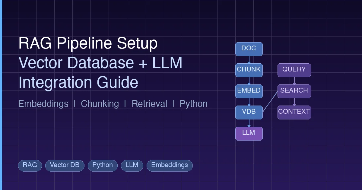
Now let’s build a complete RAG pipeline. The architecture has six stages:
Document Loading → Chunking → Embedding → Storage → Retrieval → Generation
Step 1: Document Loading
Load your source documents. In production, this might be PDFs, Markdown files, web pages, or database records.
from pathlib import Path

def load_documents(directory: str) -> list[dict]:
    """Load text documents from a directory."""
    documents = []
    for path in Path(directory).glob("**/*.md"):
        text = path.read_text(encoding="utf-8")
        documents.append({
            "text": text,
            "source": str(path),
            "filename": path.name,
        })
    return documents

docs = load_documents("./knowledge_base")
print(f"Loaded {len(docs)} documents")
Step 2: Chunking
This is where most RAG pipelines succeed or fail. The goal is to split documents into pieces that are small enough to be semantically focused but large enough to retain useful context.
Fixed-Size Chunking
The simplest approach. Split text into chunks of N tokens with overlap:
def fixed_size_chunk(text: str, chunk_size: int = 500, overlap: int = 100) -> list[str]:
    """Split text into fixed-size chunks with overlap."""
    words = text.split()
    chunks = []
    start = 0
    while start < len(words):
        end = start + chunk_size
        chunk = " ".join(words[start:end])
        chunks.append(chunk)
        start += chunk_size - overlap  # Step forward with overlap
    return chunks
Pros: Simple, predictable chunk sizes Cons: May split sentences or paragraphs mid-thought
Recursive Character Splitting
Tries to split on natural boundaries (paragraphs, sentences, words) in order:
def recursive_split(text: str, max_size: int = 500, separators: list[str] = None) -> list[str]:
    """Split text recursively on natural boundaries."""
    if separators is None:
        separators = ["\n\n", "\n", ". ", " "]

    if len(text.split()) <= max_size:
        return [text]

    for sep in separators:
        parts = text.split(sep)
        if len(parts) > 1:
            chunks = []
            current = ""
            for part in parts:
                candidate = current + sep + part if current else part
                if len(candidate.split()) > max_size and current:
                    chunks.append(current.strip())
                    current = part
                else:
                    current = candidate
            if current.strip():
                chunks.append(current.strip())
            # Recursively split any chunks that are still too large
            result = []
            for chunk in chunks:
                result.extend(recursive_split(chunk, max_size, separators))
            return result

    # Fallback: hard split by words
    return fixed_size_chunk(text, max_size)
Pros: Respects document structure, produces more coherent chunks Cons: Variable chunk sizes, slightly more complex
Semantic Chunking
Groups sentences by semantic similarity. Adjacent sentences with similar embeddings stay together; a new chunk starts when the topic shifts:
import numpy as np
from openai import OpenAI

client = OpenAI()

def get_embeddings(texts: list[str]) -> list[list[float]]:
    """Get embeddings for a batch of texts."""
    response = client.embeddings.create(
        model="text-embedding-3-small",
        input=texts
    )
    return [item.embedding for item in response.data]

def semantic_chunk(text: str, threshold: float = 0.8) -> list[str]:
    """Split text into chunks based on semantic similarity between sentences."""
    import re
    sentences = re.split(r'(?<=[.!?])\s+', text)
    if len(sentences) <= 1:
        return [text]

    embeddings = get_embeddings(sentences)

    chunks = []
    current_chunk = [sentences[0]]

    for i in range(1, len(sentences)):
        # Cosine similarity between current and previous sentence
        sim = np.dot(embeddings[i], embeddings[i-1]) / (
            np.linalg.norm(embeddings[i]) * np.linalg.norm(embeddings[i-1])
        )
        if sim < threshold:
            # Topic shift detected, start new chunk
            chunks.append(" ".join(current_chunk))
            current_chunk = [sentences[i]]
        else:
            current_chunk.append(sentences[i])

    if current_chunk:
        chunks.append(" ".join(current_chunk))

    return chunks
Pros: Highest quality boundaries, topic-aware Cons: Requires embedding API calls during chunking (slower, costs money)
Which Strategy to Use?
| Strategy | When to Use |
|---|---|
| Fixed-size | Prototyping, uniform content (logs, records) |
| Recursive | Structured documents (Markdown, HTML, code) |
| Semantic | High-quality requirements, knowledge-dense content |
Start with recursive splitting at 300-500 tokens with 50-100 token overlap. This works well for 80% of use cases.
Step 3: Embedding and Storage
Now embed your chunks and store them in a vector database. Here are complete examples with both Chroma and Qdrant.
Example with Chroma
import chromadb
from openai import OpenAI

client = OpenAI()
chroma = chromadb.PersistentClient(path="./chroma_db")

# Create or get a collection
collection = chroma.get_or_create_collection(
    name="knowledge_base",
    metadata={"hnsw:space": "cosine"}  # Use cosine similarity
)

def embed_and_store(chunks: list[dict]):
    """Embed chunks and store in Chroma."""
    texts = [c["text"] for c in chunks]

    # Batch embed (OpenAI supports up to 2048 inputs per call)
    batch_size = 2000
    all_embeddings = []
    for i in range(0, len(texts), batch_size):
        batch = texts[i:i + batch_size]
        response = client.embeddings.create(
            model="text-embedding-3-small",
            input=batch
        )
        all_embeddings.extend([item.embedding for item in response.data])

    # Store in Chroma
    collection.add(
        ids=[f"chunk_{i}" for i in range(len(chunks))],
        embeddings=all_embeddings,
        documents=texts,
        metadatas=[{"source": c["source"]} for c in chunks]
    )
    print(f"Stored {len(chunks)} chunks in Chroma")

# Prepare chunks with metadata
chunks = []
for doc in docs:
    doc_chunks = recursive_split(doc["text"], max_size=400)
    for chunk_text in doc_chunks:
        chunks.append({"text": chunk_text, "source": doc["source"]})

embed_and_store(chunks)
Example with Qdrant
from qdrant_client import QdrantClient
from qdrant_client.models import Distance, VectorParams, PointStruct
from openai import OpenAI

client = OpenAI()
qdrant = QdrantClient(url="http://localhost:6333")

# Create collection
qdrant.create_collection(
    collection_name="knowledge_base",
    vectors_config=VectorParams(
        size=1536,  # text-embedding-3-small dimensions
        distance=Distance.COSINE,
    ),
)

def embed_and_store_qdrant(chunks: list[dict]):
    """Embed chunks and store in Qdrant."""
    texts = [c["text"] for c in chunks]

    # Get embeddings
    response = client.embeddings.create(
        model="text-embedding-3-small",
        input=texts
    )
    embeddings = [item.embedding for item in response.data]

    # Create points
    points = [
        PointStruct(
            id=i,
            vector=embeddings[i],
            payload={
                "text": texts[i],
                "source": chunks[i]["source"],
            }
        )
        for i in range(len(chunks))
    ]

    # Upsert in batches
    batch_size = 100
    for i in range(0, len(points), batch_size):
        qdrant.upsert(
            collection_name="knowledge_base",
            points=points[i:i + batch_size]
        )

    print(f"Stored {len(chunks)} chunks in Qdrant")
Step 4: Retrieval
When a user asks a question, embed the query and search for similar chunks:
def retrieve(query: str, top_k: int = 5) -> list[dict]:
    """Retrieve relevant chunks for a query from Chroma."""
    # Embed the query
    response = client.embeddings.create(
        model="text-embedding-3-small",
        input=query
    )
    query_embedding = response.data[0].embedding

    # Search Chroma
    results = collection.query(
        query_embeddings=[query_embedding],
        n_results=top_k,
        include=["documents", "metadatas", "distances"]
    )

    # Format results
    retrieved = []
    for i in range(len(results["documents"][0])):
        retrieved.append({
            "text": results["documents"][0][i],
            "source": results["metadatas"][0][i]["source"],
            "score": 1 - results["distances"][0][i],  # Convert distance to similarity
        })

    return retrieved
Step 5: Generation
Combine the retrieved context with the user’s question and send it to the LLM:
def generate_answer(query: str, context_chunks: list[dict]) -> str:
    """Generate an answer using retrieved context."""
    # Build context string
    context = "\n\n---\n\n".join([
        f"[Source: {c['source']}]\n{c['text']}"
        for c in context_chunks
    ])

    response = client.chat.completions.create(
        model="gpt-4o",
        messages=[
            {
                "role": "system",
                "content": (
                    "You are a helpful assistant. Answer the user's question "
                    "based on the provided context. If the context does not "
                    "contain relevant information, say so. Always cite your "
                    "sources."
                )
            },
            {
                "role": "user",
                "content": f"Context:\n{context}\n\nQuestion: {query}"
            }
        ],
        temperature=0.1,  # Low temperature for factual responses
    )

    return response.choices[0].message.content
Putting It All Together
def rag_query(question: str) -> str:
    """Complete RAG pipeline: retrieve context and generate answer."""
    # Step 1: Retrieve relevant chunks
    chunks = retrieve(question, top_k=5)

    # Step 2: Filter low-relevance results
    relevant_chunks = [c for c in chunks if c["score"] > 0.7]

    if not relevant_chunks:
        return "I could not find relevant information to answer your question."

    # Step 3: Generate answer
    answer = generate_answer(question, relevant_chunks)

    # Step 4: Include sources
    sources = set(c["source"] for c in relevant_chunks)
    answer += f"\n\nSources: {', '.join(sources)}"

    return answer

# Usage
result = rag_query("What is our company's vacation policy?")
print(result)
Common Pitfalls and Optimization Tips
Building a RAG pipeline that works in a demo is easy. Building one that works well in production is another matter. Here are the most common mistakes and how to avoid them.
Pitfall 1: Choosing the Wrong Embedding Model
The embedding model determines the quality ceiling of your entire pipeline. A bad embedding model means bad retrieval, and no amount of prompt engineering will fix that.
Fix: Evaluate models on your actual data. Use the MTEB leaderboard as a starting point, but always test with your own queries and documents. A model that ranks #1 on general benchmarks may underperform on your specific domain.
Pitfall 2: Ignoring Chunk Overlap
Chunks without overlap can split critical information across boundaries. If a key fact spans two chunks, neither chunk contains the complete information.
Fix: Use 10-20% overlap between chunks. For 500-token chunks, use 50-100 tokens of overlap.
Pitfall 3: Not Using Metadata Filtering
Retrieving the “most similar” chunks globally may not give you the best results. If the user is asking about a specific product version, you want to filter by version first, then search.
Fix: Store rich metadata (date, category, version, author) with each chunk. Use pre-filtering to narrow the search space before similarity search. This is especially important in Qdrant, which has strong filtering support.
Pitfall 4: Stuffing Too Much Context
Retrieving 20 chunks and cramming them all into the prompt dilutes the signal. The LLM has to pick out the relevant information from a wall of text.
Fix: Retrieve more than you need, then re-rank. Use a cross-encoder or LLM-based re-ranker to score relevance, and only include the top 3-5 most relevant chunks.
def rerank(query: str, chunks: list[dict], top_k: int = 3) -> list[dict]:
    """Re-rank chunks using the LLM as a judge."""
    scored = []
    for chunk in chunks:
        response = client.chat.completions.create(
            model="gpt-4o-mini",
            messages=[{
                "role": "user",
                "content": (
                    f"Rate how relevant this text is to the question "
                    f"on a scale of 0-10.\n\n"
                    f"Question: {query}\n\n"
                    f"Text: {chunk['text']}\n\n"
                    f"Score (just the number):"
                )
            }],
            max_tokens=3,
            temperature=0,
        )
        try:
            score = float(response.choices[0].message.content.strip())
            scored.append({**chunk, "rerank_score": score})
        except ValueError:
            scored.append({**chunk, "rerank_score": 0})

    scored.sort(key=lambda x: x["rerank_score"], reverse=True)
    return scored[:top_k]
Pitfall 5: Ignoring Hybrid Search
Pure vector search misses exact keyword matches. If a user searches for “error code E-4021”, semantic search might not find the exact document because the error code is an identifier, not a semantic concept.
Fix: Combine keyword search (BM25) with vector search. Many vector databases support hybrid search natively. Qdrant and Weaviate both offer this capability.
Pitfall 6: Not Evaluating Retrieval Quality
Many teams evaluate only the final LLM output without checking whether the retrieval step returned the right documents.
Fix: Build a test set of question-answer-source triples. Measure retrieval precision and recall separately from generation quality. If retrieval is poor, no generation model will save you.
RAG vs Fine-Tuning vs Long Context
A common question: when should you use RAG versus fine-tuning versus just using a long context window? Each approach has distinct strengths.
| Approach | Best For | Limitations |
|---|---|---|
| RAG | Large, dynamic knowledge bases; source attribution needed; cost-sensitive at scale | Retrieval can miss relevant info; adds latency; requires infrastructure |
| Fine-tuning | Teaching style, format, or domain behavior; consistent output patterns | Expensive to train; does not add factual knowledge reliably; hard to update |
| Long context | Small, static document sets; one-off analysis tasks | Expensive per query; “lost in the middle” problem; context window limits |
In practice, production systems often combine approaches. You might fine-tune a model to follow your output format, use RAG to inject relevant knowledge, and use long context for complex multi-document reasoning within the retrieved set.
For most teams starting out, RAG is the right first step. It is the most cost-effective way to connect an LLM to your data, it does not require training infrastructure, and it naturally supports updating the knowledge base without retraining.
If you are building AI agents, the RAG pipeline becomes even more important. An AI agent can use RAG as a tool – calling the retrieval function as one of its available actions during an agentic loop. This pattern is widely used in production systems, including tools like Claude Code which use MCP protocol to connect to external data sources.
Production Checklist
Before deploying your RAG pipeline, verify these items:
- Embedding model evaluated on your actual data, not just benchmarks
- Chunk size tested with at least 3 different sizes (e.g., 256, 512, 1024 tokens)
- Overlap configured at 10-20% of chunk size
- Metadata stored with each chunk (source, date, category)
- Retrieval quality measured with a test set of at least 50 queries
- Re-ranking implemented if top-5 retrieval precision is below 80%
- Hybrid search enabled if your data contains identifiers, codes, or exact terms
- Rate limiting and error handling for embedding API calls
- Index backed up and recovery tested
- Monitoring in place for retrieval latency and relevance scores
Advanced Patterns
Once your basic pipeline works, consider these enhancements:
Multi-Index RAG
Maintain separate vector collections for different document types (policies, technical docs, FAQs) and route queries to the appropriate index based on intent classification.
Parent-Child Chunking
Store small chunks for precise retrieval but return the parent chunk (or full document section) for context. This gives you the precision of small chunks with the context of large ones.
Query Expansion
Rephrase the user’s query into multiple variations and retrieve results for all of them. This increases recall for ambiguous queries.
def expand_query(query: str) -> list[str]:
    """Generate query variations for better recall."""
    response = client.chat.completions.create(
        model="gpt-4o-mini",
        messages=[{
            "role": "user",
            "content": (
                f"Generate 3 different ways to ask this question. "
                f"Return only the questions, one per line.\n\n"
                f"Question: {query}"
            )
        }],
        temperature=0.7,
    )
    variations = response.choices[0].message.content.strip().split("\n")
    return [query] + [v.strip() for v in variations if v.strip()]
Caching
Cache embedding results for frequent queries. A simple hash-based cache can eliminate redundant API calls and reduce latency significantly.
Summary
A RAG pipeline is not a single technology but a system of interlocking components: document loading, chunking, embedding, vector storage, retrieval, and generation. Each component has trade-offs that affect the final output quality.
The key decisions you need to make:
- Embedding model: Start with
text-embedding-3-small, evaluate against your data - Chunking strategy: Start with recursive splitting at 400 tokens, 80-token overlap
- Vector database: Chroma for prototyping, Qdrant or Weaviate for production
- Indexing algorithm: HNSW for most cases, IVF-PQ if memory is constrained
- Retrieval depth: Retrieve 10-20 candidates, re-rank to top 3-5
Build the simple version first. Measure retrieval quality. Then optimize the weakest link. Most RAG failures are retrieval failures, and most retrieval failures are chunking or embedding model problems – not vector database problems.
For deeper exploration of how RAG fits into broader AI systems, see the Context Engineering Guide which covers how to design the information flow that AI systems receive.
Related Reading
- Build an AI Agent from Scratch in Python – Learn how to build an agentic loop that can use RAG as a tool
- AI Agent Memory Systems – How agents use vector databases for long-term memory
- MCP Protocol Explained – The protocol that connects AI tools to external data sources
- Context Engineering Guide – Design the information flow for AI systems
- MTEB Leaderboard – Compare embedding model performance (external)
- Qdrant Documentation – Official docs for the Qdrant vector database (external)
Comments
Join the discussion — requires a GitHub account